Introduction
The goal of this project is to use different classification techniques on the same dataset to compare different modeling methods. The dataset used is from a beer review website, and the models will attempt to categorize beers based on the different components of their reviews, along with the ABV of a given beer. Questions that this project will help answer are:
Modeling Differences
- Which classification method is the most accurate for this dataset?
- Which classification methods suffered from overfitting, if any?
- Which methods are easier/harder to use in R?
Beer Differences
- How does ABV differ between types of beer?
- How do beers’ reviews differ on different metrics (color, smell)?
- Can you predict what type of beer is being reviewed using just its ABV and review scores?
The Dataset
This dataset came from Kaggle. It’s a scrape of 15.8 Million reviews of beer from BeerAdvocate.com. Each review has information about what beer was reviewed where by who and when, and also has multiple different components that a beer was reviewed on.
This dataset has the following traits:
- Positive correlation between multiple variables (review components)
- Significantly more rows than columns (15.8 million rows, 14 columns)
- Mix of numerical and categorical variables
The dataset has the following variables:
| index | Index value of the review | Nominal (Categorical) |
| brewery_name | Name of the brewery that the beer came from | Nominal (Categorical) |
| brewery_id | ID of the brewery (redundant with brewery_name) | Nominal (Categorical) |
| beer_style | Broad style of the beer (American IPA, Light Lager, etc) | Nominal (Categorical) |
| beer_name | The specific name of the beer | Nominal (Categorical) |
| beer_beerid | ID of the beer (redundant with beer_name) | Nominal (Categorical) |
| review_profilename | Who wrote the review | Nominal (Categorical) |
| review_time | Date/time of the review | Continuous (Numerical) |
| review_overall | Overall rating of the beer | Discrete (Numerical) |
| review_aroma | Rating of the beer’s smell | Discrete (Numerical) |
| review_appearance | Rating of the beer’s look | Discrete (Numerical) |
| review_palate | Rating of the beer’s feel | Discrete (Numerical) |
| review_taste | Rating of the beer’s taste | Discrete (Numerical) |
| beer_abv | The beer’s alcohol by volume | Continuous (Numerical) |
Data Pre-processing
I want to find a single nominal variable to act as our target for categorization and delete the rest, because there’s generally a lot of redundancy between these variables (brewery_id is the same as brewery_name, for example). Index is unique for every value, so it’s not useful as our predicted variable. brewery_id and beer_beerid are 1:1 with other variables, so I’ll also ignore them. That leaves 4 possible nominal variables to use as our target for classification: reviewer, beer style, beer name, and brewery name. I’ll check all four of these and go with whichever has the fewest unique values, as I want to have a handful of broad categories for my classification. The other 3 will be dropped.
Libraries
library(tidyr)
library(dplyr)
library(ggplot2)
library(randomForest)
library(class)
Code
nrow(distinct(df["brewery_name"]))
nrow(distinct(df["review_profilename"]))
nrow(distinct(df["beer_name"]))
nrow(distinct(df["beer_style"]))
Output
> nrow(distinct(df["brewery_name"])) #5743 distinct values
[1] 5743
> nrow(distinct(df["review_profilename"])) #33388 distinct values
[1] 33388
> nrow(distinct(df["beer_name"])) #56857 distinct values
[1] 56857
> nrow(distinct(df["beer_style"])) #104 distinct values
[1] 104
Beer style has the fewest distinct values at 104, so it’ll be our target. Now, it’s time to prune the data. I’m dropping all nominal variables aside from beer_style, dropping review_time, and dropping all rows with NA values. I’m dropping review time because I think it’s not relevant to the question I’m asking. The dataset is large enough that there’s no need to try to salvage the rows with NA, so I’ll be simply dropping them. I’ll also cut out all duplicate rows because there’s going to be a lot of overlap between values, given the 1 to 5 star rating system that most variables follow.
Code
df <- drop_na(df) #15.8M -> 15.1M rows
df <- subset(df, select = -c(index, brewery_id, brewery_name, review_time, review_profilename, beer_name, beer_beerid))
df <- distinct(df)
Although 104 values is lower than the thousands of distinct categories for the other variables, it’s still a lot. The next step is to prune the data down even more, and I’ll be doing it by finding the 10 most common categories of beer_style, and dropping all rows that are not in one of those 10 styles.
Code
#count -> sort -> cut -> convert to vector
top_10 <- df %>% count(beer_style) %>% arrange(desc(n)) %>% slice_head(n = 10) %>% pull(beer_style)
#select only rows that have one of the 10 values
df <- df[df$beer_style %in% top_10,]
Top 10 Beers
This step reduces our data from 15.1 million rows to181k rows. As a final step for data processing, I normalize every numerical variable from 0 to 1 for any models that might need it in that format.
Code
#Normalize all continuous rows to 0 to 1
norm_func <- function(x){(x-min(x))/(max(x)-min(x))} #normalizes a given column
df <- df %>% mutate_at(colnames(df[,-4]), norm_func) #normalize every column (except beer style)
Data Visualization
After cleaning the data, the next step is to do some exploratory visualizations to help understand it better. I looked at the correlation between all remaining variables, as well as the distribution of each beer style’s overall review scores and ABV.
Code
pairs(df[sample(nrow(df),100),-4], lower.panel = NULL) #Scatterplots of all variables, using 100 random rows
ggplot(df, aes(x=review_overall, fill=beer_style)) + geom_histogram() #Histogram of overall review, colored by beer style
ggplot(df, aes(x=beer_abv, fill=beer_style)) + geom_histogram() #Histogram of abv, colored by beer style
Output
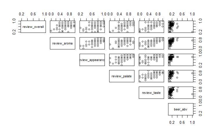
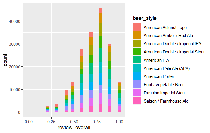
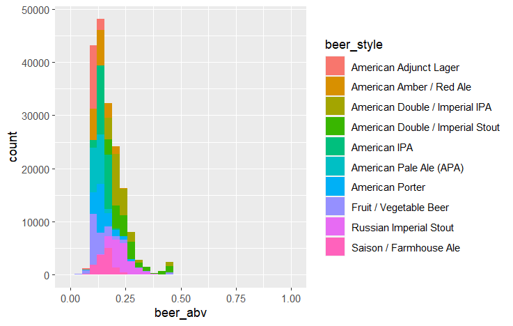
Review scores in each category have some correlation with each other, and each beer style seems to heavily overlap when it comes to review score. Beer ABV by style is more distinct, with some beer styles being noticeably higher or lower than others.
Modeling
I used an 80:20 training:testing split for this data. I chose to set it up in a way that would enable me to easily implement k fold validation, though I didn’t end up using it on this project. The two models I used were Random Forest and KNN. I used them because they’re both models that we’ve mentioned in class that are intended for classification problems and can handle continuous values.
Training/Testing Split
#To give the option for k fold validation, I'll assign each row to one of 5 folds
#Generate a vector of 1:5 on repeat that is nrows long, then randomize its order and assign it to a new column
set.seed(4)
df$beer_style <- as.factor(df$beer_style) #Convert beer_style to a factor
df <- df %>% mutate(fold = sample(rep(1:5, length.out = nrow(df)),nrow(df),replace=FALSE))
#Get our training and testing sets (exclude fold column)
train = df[df$fold != 1,-8]
test = df[df$fold == 1,-8]
Random Forest
rf <- randomForest(beer_style ~ ., data = train)
print(rf)
rf_predictions <- predict(rf, test)
KNN
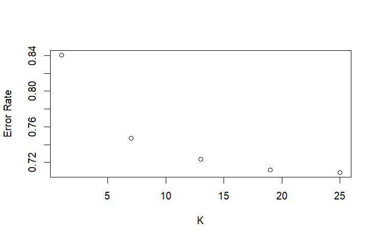
#Choosing K value
#First Pass
i <- 1
knn_errors <- c()
for (i in 0:4){ #First check: 5 values from 1 to 25
j = 1 + 6 * i
predict <- knn(train=train[,-4], test=test[,-4], cl=train[,4], k=j)
error_rate <- mean(predict != test[,4])
knn_errors[i+1] = error_rate
}
plot(seq(1, 25, 6), knn_errors, xlab = "K", ylab = "Error Rate") #Elbow point looks to be somewhere between 1 and 13
#Second Pass
i <- 1
knn_errors <- c()
for (i in 0:6){ #Second Check: 5 values from 1 to 13
j = 1 + 2 * i
predict <- knn(train=train[,-4], test=test[,-4], cl=train[,4], k=j)
error_rate <- mean(predict != test[,4])
knn_errors[i+1] <- error_rate
}
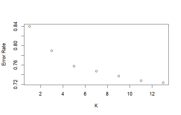
plot(seq(1, 13, 2), knn_errors, xlab = "K", ylab = "Error Rate") #Elbow point at 5
#Make final model on best K value
knn_predictions <- knn(train=train[,-4], test=test[,-4], cl=train[,4], k=5)Output
Due to the large size of this dataset, training the Random Forest was extremely memory intensive. Random Forest’s complexity scales at n*log(n) complexity, while KNN scales at n, making it much slower at a dataset of this scale. However, KNN was also slow due to testing multiple K values, so I optimized the search for the best K value by checking Ks at larger intervals before iterating every K value in a smaller range. Another issue I had with KNN was the “too many ties” error, which comes from having too many neighbors the same distance from the point we’re evaluating. I fixed this error by creating a different training set for KNN that was just the unique values of the base training set.
Evaluation
To evaluate this model, I used accuracy, precision, recall, and F1 score because they’re standard evaluation metrics in classification problems. Because this is a multi-class problem, I had to find the precision and recall for each class and average them to get the overall precision and recall of the model.
Code
#Evaluation
#Create two confusion matrices
rf_conf_matrix <- table(rf_predictions, test$beer_style)
print(rf_conf_matrix)
knn_conf_matrix <- table(knn_predictions, test$beer_style)
print(knn_conf_matrix)

#Accuracy
rf_accuracy <- sum(diag(rf_conf_matrix)) / sum(rf_conf_matrix)
knn_accuracy <- sum(diag(knn_conf_matrix)) / sum(knn_conf_matrix)

#Precision
rf_precision_per_class <- c()
knn_precision_per_class <- c()
for (i in 1:10) {
  rf_precision_per_class[i] <- rf_conf_matrix[i,i] / sum(rf_conf_matrix[i,])
  knn_precision_per_class[i] <- knn_conf_matrix[i,i] / sum(knn_conf_matrix[i,])
}
rf_precision <- mean(rf_precision_per_class)
knn_precision <- mean(knn_precision_per_class)

#Recall
rf_recall_per_class <- c()
knn_recall_per_class <- c()
for (i in 1:10) {
  rf_recall_per_class[i] <- rf_conf_matrix[i,i] / sum(rf_conf_matrix[,i])
  knn_recall_per_class[i] <- knn_conf_matrix[i,i] / sum(knn_conf_matrix[,i])
}
rf_recall <- mean(rf_recall_per_class)
knn_recall <- mean(knn_recall_per_class)

#F1 Score
rf_f1 <- (2*rf_precision*rf_recall)/(rf_precision+rf_recall)
knn_f1 <- (2*knn_precision*knn_recall)/(knn_precision+knn_recall)
Output
| Random Forest | KNN | |
| Accuracy | 0.377 | 0.242 |
| Precision | 0.357 | 0.219 |
| Recall | 0.354 | 0.233 |
| F1 Score | 0.355 | 0.226 |
Both models were not very good at predicting beer style based on reviews, though random forest was consistently better on every metric.
Findings
I discovered that review scores, when broken down by review metric, have some, though not much, ability to predict a beer’s style when combined with ABV. Another question I wanted to ask was which method was easier to train a model for in R, given the same dataset. I found Random Forest to be the easier method, as proven by how much shorter its code block is compared to KNN. The lengths of each code block don’t show it, but I also spent longer troubleshooting KNN compared to Random Forest.
Impact
Although the impact isn’t massive, I can say for sure that in the future I’ll lean toward using Random Forest instead of KNN. RF was easier to get running, and performed better.
References
I mainly referred to the documentation for my methods, but I also used some other sources. Here is every source I used when coding this.
